

Guide
Monte Carlo backtest: what resampling your trades can and cannot tell you
 Tommy J.Founder, RoboticEA
A Monte Carlo backtest takes the trades your strategy already made and re-deals them a thousand different ways — reordered, resampled, thinned out, made slightly more expensive — to ask how much of the result was the strategy and how much was the luck of the sequence. It is a genuinely useful test. It is also routinely sold as something it is not. This post runs our own Monte Carlo code on a real 456-trade backtest and shows you, chart by chart, exactly what it can and cannot tell you.
The short answer
Definition
What a Monte Carlo backtest is
A normal backtest gives you one path: the trades in the order the market produced them, one equity curve, one maximum drawdown. But that order is partly an accident. Had the same 456 trades arrived in a different sequence, the account would have ended at the same place — and visited very different lows on the way.
A Monte Carlo simulation in trading replaces “the one path” with a distribution of plausible paths built from the same raw material. You take the list of per-trade returns, apply a random perturbation, rebuild the equity curve, record its return and drawdown, and repeat — a thousand times or more. Then you read percentiles instead of a single number: “in 95% of simulations the drawdown stayed above X” is a much more honest planning figure than “the drawdown was Y”.
The key word is same raw material. Every simulated path is assembled from trades that already happened in the backtest window. Hold on to that — it is the source of both the method’s strength and its blind spot.
Mechanics
The four ways to perturb a trade list
There is no single “Monte Carlo”; there are several perturbations that answer different questions. Our implementation — packages/validation/src/montecarlo.ts in the RoboticEA codebase — has four, and they are worth describing precisely, because most tools do not say which ones they apply.
| Method | What it does to the trade list | Question it answers |
|---|---|---|
| Shuffle | Same trades, random order (Fisher–Yates) | How lucky was the drawdown? |
| Bootstrap | Draw N trades with replacement — some repeat, some vanish | How wide is the range of outcomes from this edge? |
| Omission | Drop each trade with probability 10% | Did a handful of trades carry the result? |
| Slippage | Subtract a random half-normal cost from every trade | How thin is the margin over friction? |
Two details matter more than they look. First, when all four are combined, the order is fixed: bootstrap, then omission, then shuffle, then slippage — membership first, ordering second, cost last. Second, the slippage perturbation is one-sided. It subtracts the absolute value of a Gaussian draw, so it can only ever make a trade worse; on average it costs about 0.024% of equity per trade. A symmetric “noise” model would let simulated slippage improve results half the time, which no broker has ever done for anyone.
From each simulated curve the code records three numbers — compounded total return, maximum drawdown and Sharpe ratio — and summarises each as a mean, median and 95% interval (the 2.5th and 97.5th percentiles). It also reports one tail figure on its own: the 5th-percentile maximum drawdown, which is what its pass/fail rule consumes.
A real run
A Monte Carlo simulation on a real backtest
Illustrations with made-up trades prove nothing, so here is a real one: a deliberately plain trend-follower — exponential Hull MA(30) crossover, ATR(14) x 2.5 stop, exit on opposite signal, 1% risk per trade (ATR-based sizing) — run by our engine on EURUSD H1 for 2023, on recorded market bars (rbar-m5:EURUSD_H1_2023). It is one of the runs from our MetaTrader 5 parity work, where the same strategy was also executed in MT5’s Strategy Tester and 443 of its 456 trades were matched bar-for-bar (96.3% entry-bar agreement).
456
trades
+43.1%
return, 2023
−7.3%
max drawdown
1.35
profit factor
One caveat up front, because it matters: parity runs are executed with trading costs switched off (zero), since their job is to compare fills with MT5, not to estimate profit. So the +43.1% is a frictionless figure and should not be read as what this strategy would have earned. For this post that is almost an advantage: it lets us see how much damage Monte Carlo’s own slippage perturbation does on its own. We fed the trade list through the production parser and the production Monte Carlo, with the seed derivation the pipeline uses, and wrote every result to a file the charts below are drawn from.
Shuffle: the return never moves, the drawdown does
This is the result most people do not expect. Compounding is multiplication, and multiplication does not care about order, so a pure shuffle cannot change the final return at all — every one of the 1,000 paths above finishes at +43.1%. Any tool that shows you a “Monte Carlo range of returns” from shuffling alone is showing you something else, usually fixed-size position maths or a bootstrap under a different name.
What shuffling does reveal is how flattering the real sequence was. Rebuilt from closed trades, the original order drew down −7.1%. In 84.7% of reorderings the drawdown was deeper than that; the median was −9.1% and one ordering in twenty went past −13.9%. In other words, 2023 served this strategy its trades in an unusually kind order. If you size the account to survive the drawdown you saw, you are sizing to the lucky case.
Bootstrap: the range of outcomes from the same edge
The bootstrap is the method that actually produces a return range, because it changes which trades you get, not just their order. A H1 trend-follower with a 32% win rate lives on a minority of large winners — the single largest trade here was 22% of the net profit — so drawing a few more or a few fewer of them swings the result a long way. A 95% interval running from +1.5% to +107.7% around one real +43.1% year is the honest size of the uncertainty in a single backtest of 456 trades.
Omission and slippage
| Method alone | Median return | 95% range | Median max DD | 5th-pct DD |
|---|---|---|---|---|
| Shuffle | +43.1% | +43.1% … +43.1% | −9.1% | −13.9% |
| Bootstrap | +43.8% | +1.5% … +107.7% | −9.1% | −16.0% |
| Omission (10%) | +37.9% | +22.7% … +52.7% | −6.8% | −8.9% |
| Slippage | +28.3% | +27.4% … +29.3% | −8.1% | −8.3% |
Omission is the “was it a few lucky trades?” test. Dropping a random tenth of the trades left the median at +37.9% and never turned the year into a loss — the edge here is spread across many trades rather than parked in three. Slippage is the sobering one. A noise term averaging 0.024% of equity per trade sounds like nothing, but over 456 trades it took the median from +43.1% to +28.3% — 14.8 points of return gone to friction alone. High-frequency strategies live or die on that line, which is exactly why our real backtests charge the recorded spread inside every trade instead of approximating it afterwards.
The full simulation
All four at once: the Monte Carlo distribution
Our pipeline’s default applies all four perturbations in every iteration. This is the distribution it produces for the same 456 trades:
+24.5%
median simulated return
−9% … +73%
95% interval
8.7%
of simulations lost money
−19.4%
5th-percentile drawdown
Read the two charts together and the picture is coherent. The strategy has a real edge in these trades — the bulk of the distribution is positive — but the backtest you would have been shown is near the generous end of what those trades could produce, on both return and drawdown. Planning around the median (+24.5%, −10.5% drawdown) rather than the actual result is the practical lesson, and it is the right one.
Sizing
Risk of ruin and the Monte Carlo drawdown gate
The most useful thing a Monte Carlo simulation does is turn “how bad can it get?” into a frequency. From the combined run:
| Drawdown at least this deep | Share of simulations |
|---|---|
| −10% | 55.4% |
| −15% | 17.8% |
| −20% | 3.5% |
| −25% | 0.9% |
Our validation code turns that tail into a hard gate: the 5th-percentile drawdown must be shallower than −25%. This run clears it, at −19.4%. In risk-of-ruin terms — the chance of hitting a loss you cannot or will not recover from — that is the kind of statement a trader can act on: if a −25% drawdown would end the account (or your nerve), 0.9% of simulated years got there.
Two honest limits on that number. First, a Monte Carlo rebuilds the equity curve from closed trades only. Our engine, which marks open positions to market, measured this run’s drawdown at −7.28%; the closed-trade curve says −7.12%. The gap is small here and can be large for strategies that sit through deep open losses, so a trade-list Monte Carlo systematically understates drawdown. Second, the frequencies assume the future deals from the same deck. That is the assumption the next section is about.
The limit
What Monte Carlo cannot tell you
Every simulated path above was built from the 456 trades of 2023. If 2023 was a year that happened to suit this rule — and a strategy is usually chosen because its backtest window suited it — then every simulation inherits that luck. Monte Carlo can tell you the trades were not a fluke of ordering. It cannot tell you whether the market will keep producing trades like them.
That is not a theoretical worry. It is the single largest effect we have measured. In one study we took the top 25 strategies by in-sample return and ran each on 12 instruments:
+15.25% → −18.27%
top-ranked H1 strategies at home, then on instruments they were not chosen on
Top 25 by in-sample return, transplanted to 12 instruments (95% interval −19.21% to −14.27%). Rank correlation between instrument pairs: ρ = 0.210. Source: robots-study.json, docs/audits/stacking-and-intrabar-2026-08-08.md.
And moving through time instead of instruments gives the same answer. In our EURUSD study, the top 25 badged strategies selected on 2018–2023 had a median compounded in-sample return of +656%. On 2024–2026, years they were never selected on, the median was −56%, and 8% of them made money at all.
A Monte Carlo run on any of those in-sample trade lists would have resampled precisely the trades that made them look good. It has no access to the years and instruments they failed on, because those trades are not in the list. Resampling cannot manufacture evidence that was never collected — which is why a Monte Carlo pass is not an overfitting test, however often it is marketed as one. There are two more structural blind spots:
- Trades are treated as independent. Bootstrap and shuffle assume any trade could follow any other. Real trades cluster: a trend-follower’s losses arrive together in ranging months. Breaking those clusters tends to make the simulated worst case milder than reality.
- The cost model is whatever the backtest had. Slippage noise is a perturbation around the trades you have. If the backtest never charged the real spread, Monte Carlo will not add it — our own example is the proof, with a frictionless +43.1% that the slippage arm alone cut to +28.3%.
Robustness testing
Monte Carlo vs walk-forward optimization vs per-year validation
Robustness testing for a trading strategy is really three different questions, and each method answers one of them:
| Method | Uses new market data? | Answers |
|---|---|---|
| Monte Carlo | No — reuses the backtest's own trades | Was the result, and especially the drawdown, a lucky sequence? |
| Walk-forward analysis / optimization | Yes — tests each fold on the window after it | Does a rule fitted on the past keep working on the next period? |
| Per-year validation | Yes — a separate backtest for every calendar year | In which market years does this exact rule make or lose money? |
Walk-forward optimization re-fits parameters on a rolling in-sample window and scores them on the out-of-sample window that follows. Our code contains a walk-forward stage as well (rolling or anchored folds, requiring the out-of-sample periods to retain at least 60% of in-sample performance), alongside the Monte Carlo described above and a blended robustness score.
We should be precise about what the product actually runs. When you press Validate in RoboticEA today, it does not run that Monte Carlo pipeline. It runs the strategy as a separate, real backtest on every calendar year of data we hold for its instrument and timeframe, with the same cost model and starting balance, and lays the results out as a grid — return, drawdown, and a profitable-versus-losing tally, each year replayable trade by trade. The Monte Carlo and walk-forward code still exists in our repository; per-year validation is what ships.
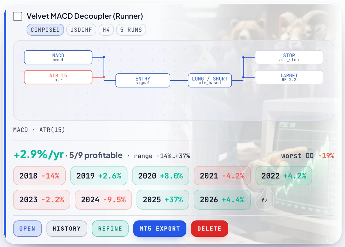
The reason to prefer per-year re-runs as the default is the section above. A year-by-year grid generates new trades on market conditions the strategy may never have been tuned on, so it can expose exactly the failure Monte Carlo is blind to: a rule that was great in its selection year and ordinary or worse everywhere else. A card with one brilliant chip and six red ones tells you more about overfitting than any number of reshuffles of the brilliant year.
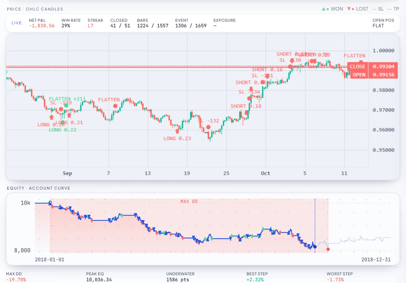
The two methods do combine well, in that order. Use per-year (or walk-forward) results to decide whether the edge is real at all; only then use a Monte Carlo of the trades you believe in to decide how much drawdown to plan for and how much to risk per trade. Running them the other way round — a tight Monte Carlo band on an in-sample winner — produces confidence without evidence.
See every year, not one lucky one
RoboticEA re-runs each strategy on every year of data separately, with the real recorded spread charged, and keeps the losing years on the card. Free account, no card, MetaTrader 5 export included.
Practical
How to run a Monte Carlo backtest yourself, free
You do not need special software — a free Monte Carlo simulation calculator is a spreadsheet or thirty lines of script. The steps that matter:
- Start from per-trade returns, not P&L. Divide each trade’s profit by the account balance before it opened. That keeps compounding honest when trades are reordered. Export the trade list from your backtester’s report (MT5’s Strategy Tester report lists every deal).
- Choose the perturbation for your question. Shuffle for drawdown sequence risk; bootstrap for a range of returns; omission to see if a few trades carry the result; a one-sided cost per trade for friction. Do not expect shuffle alone to move the final return — it cannot.
- Run at least 1,000 iterations with a fixed seed. So the answer does not change every time you open the file.
- Report percentiles, not the mean. Median return, the 5th-percentile drawdown, and the share of simulations that lost money.
- Size from the tail. Pick a risk per trade at which the 5th-percentile drawdown is one you could live through — then remember that a trade-list simulation understates open-trade drawdown, and leave room.
- Then test something it cannot. Run the same rule on years and instruments it was not chosen on. If you want that part done for you, that is what per-year validation in RoboticEA does, and how our selection studies were measured.
One last reading tip for anyone handed a Monte Carlo report by a seller: ask which perturbations were applied, to which trades, and whether those trades came from the same window the strategy was chosen on. A narrow band around an in-sample result is a statement about the sequence, not about the future.
FAQ
Questions, answered
What is a Monte Carlo backtest?
A Monte Carlo backtest takes the trades a strategy already made in a backtest and rebuilds the equity curve hundreds or thousands of times with the trades perturbed — reordered (shuffle), resampled with replacement (bootstrap), randomly dropped (omission) or made slightly more expensive (slippage). Instead of one return and one drawdown you get a distribution, and you read percentiles: the median outcome, the 95% range, and the 5th-percentile drawdown. Every simulated path is built from the same trades, which is both its strength and its main limitation.
Does shuffling the trade order change the total return?
No. Compounded return is a product of (1 + each trade's return), and multiplication does not depend on order, so a pure shuffle leaves the final return identical in every iteration. In our real example, all 1,000 shuffled paths ended at exactly +43.1%. What shuffling changes is the drawdown: the median shuffled drawdown was −9.1% against −7.1% in the original order, and 84.7% of orderings drew down deeper. A Monte Carlo range of returns has to come from bootstrap, omission or cost perturbations, not from shuffling.
How many Monte Carlo simulations do I need?
At least 1,000 iterations, with a fixed random seed so the result is reproducible. Our implementation defaults to 1,000 iterations, draws every random number from one seeded generator, and reports 95% intervals (the 2.5th and 97.5th percentiles) plus the 5th-percentile maximum drawdown. More iterations make the tails smoother; they do not make the answer more true, because every iteration reuses the same underlying trades.
Can Monte Carlo simulation detect overfitting?
No. Monte Carlo only resamples trades from the backtest window, so if a strategy was selected because that window suited it, every simulation inherits the same luck. In our holdout studies the top 25 H1 strategies by in-sample return went from +15.25% at home to −18.27% on instruments they were not chosen on, and a top-25 EURUSD selection with a median in-sample return of +656% had a median of −56% on later years. A Monte Carlo of the in-sample trades cannot see either effect, because the failing trades are not in the list. Only testing on data the strategy was not selected on can.
How do you estimate risk of ruin with Monte Carlo?
Count how often the simulated maximum drawdown crosses a loss you could not recover from. In our example with all four perturbations, 3.5% of 1,000 simulations drew down 20% or more and 0.9% reached 25%, with a 5th-percentile drawdown of −19.4% — at the run's own 1% risk per trade. Those frequencies scale with position size, and a trade-list simulation rebuilds the curve from closed trades only, so it understates open-trade drawdown. Treat the tail as a floor on the risk, not a ceiling.
Does RoboticEA run a Monte Carlo on my strategy?
No. Our codebase contains a Monte Carlo stage — the one used for every figure in this post — but when you press Validate the product runs per-year validation instead: the strategy is re-run as a separate real backtest on every calendar year of data we hold for its instrument and timeframe, and the results are shown as a year-by-year grid with the losing years kept. That tests something Monte Carlo cannot: how the same rule behaves in market years it may never have been chosen on.
Every figure from the example run is reproducible: the trade list is the engine’s own output for ehma_cross on EURUSD H1 2023 (rbar-m5:EURUSD_H1_2023, engine 0.1.0, costs zero), and the simulations are 1,000 iterations of our production Monte Carlo at seed 1934318733. Every figure on this page is a historical simulation; none of it is a forecast.
Keep reading
Do forex robots actually work?
The selection studies quoted above: why the best in-sample strategies stop winning when moved.
What a walk-forward test does to EURUSD winners
The EURUSD study behind the time-holdout figure, split by split.
How accurate is the MT5 Strategy Tester?
The parity work this post's example run came from, on real ticks.
What the real spread does to a backtest
Costs off versus costs on, cell for cell — the thing Monte Carlo slippage only approximates.
How per-year validation works
Every strategy re-run on each year separately, with the losing years kept.
Test a strategy yourself
Free account, no card. Backtest per year with real recorded spread and export to MT5.